Market Basket Analysis allows us to find groups of items that are
frequently bought together, an useful information for a variety of
reasons, both commercially and operationally.
- data preparation and application of the algorithm
Given that its algorithmic implementation is very resource-hungry, we
will here concentrate on non duplicated purchases made in
Belgium, considering both confirmed and cancelled
invoices,
df %>%
  filter(Country == "Belgium") %>%
  distinct()
having access then to 56 of them for 479
distinct stock codes.
df %>%
  filter(Country == "Belgium") %>%
  distinct() %>%
  summarise("Number of Invoices" = n_distinct(Invoice),
            "Number of Distinct Stock Codes" = n_distinct(StockCode))
In order to feed it into the algorithm, we need to change the data
frame into a transaction format, where we have a row for every invoice
and as many additional columns as the number of distinct stock codes.
The values in the cell are logical values that specify on whether the
invoice contains (TRUE) or doesn’t contain
(FALSE) that particular stock code.
(dftr <- df %>%
   filter(Country == "Belgium") %>%
   distinct() %>%
   count(Invoice, StockCode) %>%
   mutate(n = TRUE) %>%
   tidyr::pivot_wider(id_cols = Invoice, names_from = StockCode, values_from = n, values_fill = FALSE))
library(arules)
dftr <- dftr %>%
    select(-Invoice)
tr <- as(dftr, "transactions")
#we transform the data frame into a "transactions" class
rules <- apriori(tr, conf = 0, minlen = 2)
#conf = 0 to not filter out any rules, minlen = 2 to not have rules with one side empty
- rules’ filtering
After its application, the algorithm returns the following
21 “rules”, that must be read as
“if StockCode1 is being bought, then
(=>) there is a chance that StockCode2 will
be bought as well (in the same invoice)”
tibble(lhs = labels(lhs(rules)),
       rhs = labels(rhs(rules)),
       rules@quality) %>%
  mutate(" " = "=>", .after = "lhs") %>%
  rename(StockCode1 = lhs, StockCode2 = rhs)
This “chance” is expressed by a number of metrics
(support, confidence, coverage
and lift), plus we also have the number of times that
particular association of stock codes exists, count. Notice
how we have many one-to-one associations (22551 => 22554
and then 22554 => 22551) but for some of them the values
in the metrics are different (like for 22630 => 22629 /
22629 => 22630 in confidence and
coverage).
The metrics are what we use to filter the rules, and we will here
explain their meanings, using the first one
(22551 => 22554)
tibble(lhs = labels(lhs(rules)),
       rhs = labels(rhs(rules)),
       rules@quality) %>%
  mutate(" " = "=>", .after = "lhs") %>%
  rename(StockCode1 = lhs, StockCode2 = rhs) %>%
  slice(1)
as an example:
support is the percentage of times all stock codes of
the rule occur together in the same invoice over the totality of
invoices, so we get 0.1785714 which is 10 /
56
df %>%
  filter(Country == "Belgium") %>%
  distinct() %>%
  count(Invoice, StockCode) %>%
  mutate(n = TRUE) %>%
  tidyr::pivot_wider(id_cols = Invoice, names_from = StockCode, values_from = n) %>%
  select(Invoice, `22551`, `22554`) %>%
  filter(if_all(everything(), ~ !is.na(.x)))
confidence is the percentage of times the association
happens, that is with StockCode1 in an invoice there is
also StockCode2, and that happens for 10
invoices out of 12, the 0.8333333
df %>%
  filter(Country == "Belgium") %>%
  distinct() %>%
  count(Invoice, StockCode) %>%
  mutate(n = TRUE) %>%
  tidyr::pivot_wider(id_cols = Invoice, names_from = StockCode, values_from = n, values_fill = FALSE) %>%
  select(Invoice, `22551`, `22554`) %>%
  filter(`22551`)
coverage is the percentage of times
StockCode1 is present in the data set, so here its value is
0.2142857 (12 out of 56)
df %>%
  filter(Country == "Belgium") %>%
  distinct() %>%
  count(Invoice, StockCode) %>%
  mutate(n = TRUE) %>%
  tidyr::pivot_wider(id_cols = Invoice, names_from = StockCode, values_from = n) %>%
  select(Invoice, `22551`) %>%
  filter(`22551`)
lift is calculated by dividing the
confidence of the rule by the percentage of times
StockCode2 occurs in the data set, so
0.8333333 / (12 / 56), that
equals 3.888889
df %>%
  filter(Country == "Belgium") %>%
  distinct() %>%
  count(Invoice, StockCode) %>%
  mutate(n = TRUE) %>%
  tidyr::pivot_wider(id_cols = Invoice, names_from = StockCode, values_from = n) %>%
  select(Invoice, `22554`) %>%
  filter(`22554`)
It measures the “strength” of the rule, so, higher the
lift, higher the number of times StockCode1
and StockCode2 occur together in a non fortuitous way,
meaning that the purchase of StockCode1 really improves the
chances of StockCode2 being bought. For this reasons, we
want it to be higher than 1.5, given that having it under
1 means that the two stock codes are substitutes of one
another, while it equal to 1 means that the two stock codes
are independently bought.
Given that all of our rules have a strong lift, the
factors by which we filter are confidence (to have
trustworthy rules)
tibble(lhs = labels(lhs(rules)),
       rhs = labels(rhs(rules)),
       rules@quality) %>%
  mutate(" " = "=>", .after = "lhs") %>%
  rename(StockCode1 = lhs, StockCode2 = rhs) %>%
  arrange(desc(confidence))
and coverage (to have rules that happen frequently).
tibble(lhs = labels(lhs(rules)),
       rhs = labels(rhs(rules)),
       rules@quality) %>%
  mutate(" " = "=>", .after = "lhs") %>%
  rename(StockCode1 = lhs, StockCode2 = rhs) %>%
  arrange(desc(coverage))
Cutoff values could be 0.75 for confidence,
meaning that the rule is true 3 times out of
4, and 0.20 for coverage meaning
that StockCode1 is present every 5 stock
codes.
With these values, we preserve 3 rules,
tibble(lhs = labels(lhs(rules)),
       rhs = labels(rhs(rules)),
       rules@quality) %>%
  mutate(" " = "=>", .after = "lhs") %>%
  rename(StockCode1 = lhs, StockCode2 = rhs) %>%
  filter(confidence >= 0.75 &
           coverage >= 0.2)
for 4 distinct stock codes:
df %>%
  filter(StockCode %in% c("22551", "22554", "22629", "22630")) %>%
  distinct(StockCode, Description)
- analysis of the results
The 4 stock codes have, in the Belgian subset, these
characteristics,
df %>%
  filter(Country == "Belgium" &
           StockCode %in% c("22551", "22554", "22629", "22630")) %>%
  group_by(StockCode) %>%
  summarise("Number of Invoices" = n_distinct(Invoice),
            "Median Quantity" = median(abs(Quantity)),
            "Median Price" = median(Price))
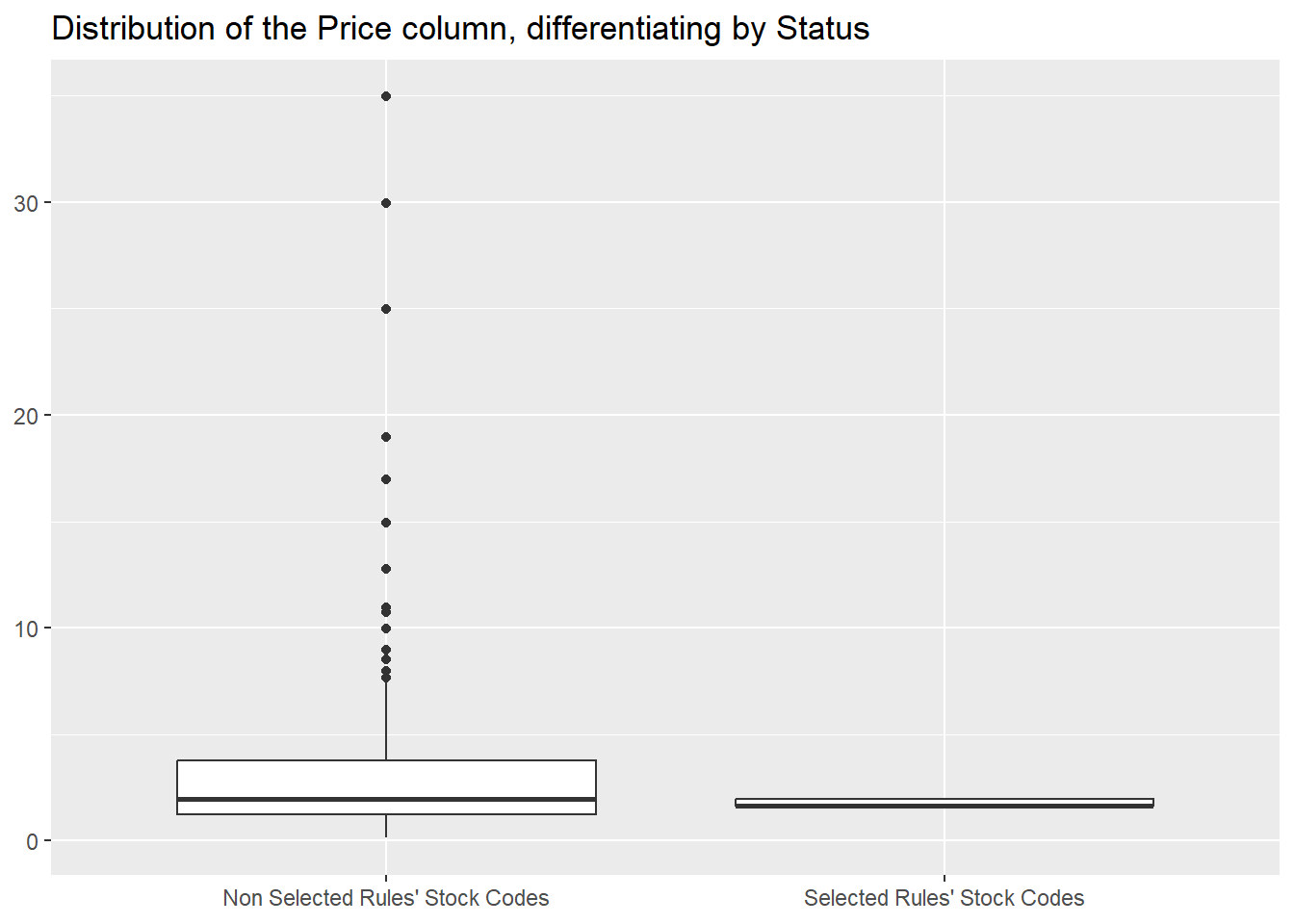
that we can compare to the rest of the inventory, where we can see
that they are generally cheaper
library(ggplot2)
df %>%
  filter(Country == "Belgium") %>%
  mutate(Status = if_else(StockCode %in% c("22551", "22554", "22629", "22630"), "Selected Rules' Stock Codes", "Non Selected Rules' Stock Codes")) %>%
  ggplot(aes(Status, Price)) +
  geom_boxplot() +
  labs(x = NULL,
       y = NULL,
       title ="Distribution of the Price column, differentiating by Status")
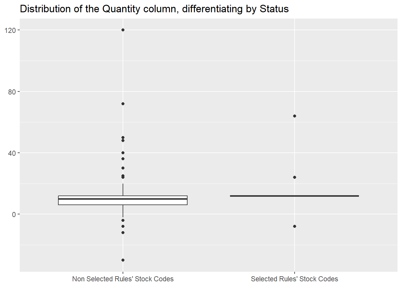
and that they are bought in roughly the same quantities.
df %>%
  filter(Country == "Belgium") %>%
  mutate(Status = if_else(StockCode %in% c("22551", "22554", "22629", "22630"), "Selected Rules' Stock Codes", "Non Selected Rules' Stock Codes")) %>%
  ggplot(aes(Status, Quantity)) +
  geom_boxplot()  +
  labs(x = NULL,
       y = NULL,
       title ="Distribution of the Quantity column, differentiating by Status")
Finally, let’s compare the revenues they generate with the overall
country revenues.
df %>%
  filter(Country == "Belgium" &
           !str_starts(Invoice, "C")) %>%
  summarise("Belgian Revenues" = sum(Quantity * Price)) %>%
  bind_cols(df %>%
              filter(Country == "Belgium" &
                       StockCode %in% c("22551", "22554", "22629", "22630") &
                       !str_starts(Invoice, "C")) %>%
              summarise("Selected Rules' Revenues" = sum(Quantity * Price))) %>%
  mutate("In Percentage" = formattable::percent(`Selected Rules' Revenues` / sum(`Selected Rules' Revenues`, `Belgian Revenues`)))
- main takeaways and further developments
We here applied an association rules algorithm to a subset of our
data, finding, after some filtering, 4 stock codes that, in
pairs of 2, are frequently bought together.
Different subsets can be examined afterwards or, with more processing
power, we can run the same analysis on the whole data frame.