Building from the previous document, where we removed the rows not
pertaining to actual transactions, we continue to clean the data frame,
concentrating here on missing values and possible duplicated rows.
- missing values (NAs)
In R missing values are coded as NA (Not Available), and
they signify that, for whatever reason, a value in a cell has not been
imputed like here for the Description and
CustomerID columns.
df %>%
  filter(if_any(everything(), ~ is.na(.x))) %>%
  slice(4)
Our original data frame had this distribution of missing values.
df %>%
  summarise(across(everything(), ~ sum(is.na(.x)))) %>%
  tidyr::pivot_longer(cols = everything()) %>%
  left_join(df %>%
              summarise(across(everything(), ~ formattable::percent(mean(is.na(.x))))) %>%
              tidyr::pivot_longer(cols = everything()), by = "name") %>%
  rename(Column = name, "Total Number" = value.x, Percentage = value.y) %>%
  arrange(desc(`Total Number`))
While the one resulting from the cleaning procedure of the last
document this one,
df_cleaned %>%
  summarise(across(everything(), ~ sum(is.na(.x)))) %>%
  tidyr::pivot_longer(cols = everything()) %>%
  left_join(df_cleaned %>%
              summarise(across(everything(), ~ formattable::percent(mean(is.na(.x))))) %>%
              tidyr::pivot_longer(cols = everything()), by = "name") %>%
  rename(Column = name, "Total Number" = value.x, Percentage = value.y) %>%
  arrange(desc(`Total Number`))
from where we can see that the manipulations we applied to the
original data frame removed some NAs in the
CustomerID column and all of them in the
Description one, while adding 308 in
Country, as we modified the Unspecified value
to NA.
We also have to mention that removing NAs can modify
tables seen in the last section of the previous document: more
specifically this one where, for some countries, the number of customers
decreases of one digit if we remove the missing values in the
CustomerID column.
df_cleaned %>%
  count(Country, wt = n_distinct(CustomerID), sort = TRUE, name = "Number of Customers") %>%
  full_join(df_cleaned %>%
              filter(!is.na(CustomerID)) %>%
              count(Country, wt = n_distinct(CustomerID), name = "Number of Customers after Removing NAs"), by = "Country")
That is because NAs are counted as one value, like they
are one actual CustomerID value, as we can see in the
following table where we show their distribution for
EIRE.
df_cleaned %>%
  filter(Country == "EIRE") %>%
  count(CustomerID, name = "Number of Occurrences")
From the previous table, we notice as well how we lost three
countries by removing NAs (Bermuda,
Hong Kong and Lebanon), as evidently these
three countries only had those in the CustomerID
column.
- CustomerID
Getting back to the table with the distribution of NAs,
CustomerID is obviously very concerning, as its missing
values amount to 20% of the all data frame. Removing them
would cause a big loss in information and modeling power so we would
have to decide on a case per case basis depending on the type of
analysis.
Let’s see if there are some patterns for these missing values, as a
way to find causes or common factors.
Every Invoice value has either the
CustomerID’s one present or missing for all of its rows so
we exclude an error in data entry like that the value of
CustomerID has, for example, been imputed only for the
first row of each value of Invoice and not for the
subsequent others.
df_cleaned %>%
  group_by(Invoice) %>%
  summarize("Percentage of NAs" = formattable::percent(mean(is.na(CustomerID)))) %>%
  count(`Percentage of NAs`, name = "Number of Invoices")
Let’s see if there are some values in the other characters columns
for which the CustomerID value is always missing.
We start with StockCode (together with
Description, to give some context).
df_cleaned %>%
  group_by(StockCode, Description) %>%
  summarize("Percentage of NAs" = formattable::percent(mean(is.na(CustomerID))),
            "Number of Occurrences" = n(), .groups = "drop") %>%
  filter(`Percentage of NAs` == 1) %>%
  arrange(desc(`Number of Occurrences`))
Then Description alone.
df_cleaned %>%
  group_by(Description) %>%
  summarize("Percentage of NAs" = formattable::percent(mean(is.na(CustomerID))),
            "Number of Occurrences" = n()) %>%
  filter(`Percentage of NAs` == 1) %>%
  arrange(desc(`Number of Occurrences`))
And finally Country, where we rediscover the three
countries mentioned ealier,
df_cleaned %>%
  group_by(Country) %>%
  summarize("Percentage of NAs" = formattable::percent(mean(is.na(CustomerID))),
            "Number of Occurrences" = n()) %>%
  filter(`Percentage of NAs` == 1) %>%
  arrange(desc(`Number of Occurrences`))
three countries that don’t contribute much though to the overall
number of NAs in the CustomerID column (only
118 rows out of 103183).
df_cleaned %>%
  filter(Country %in% c("Bermuda", "Hong Kong", "Lebanon"))
Also the countries with a percentage of NAs in the
CustomerID column less than 100% don’t
communicate a lot, besides the highest percentages belonging to
countries outside of Europe.
df_cleaned %>%
  group_by(Country) %>%
  summarize("Percentage of NAs" = formattable::percent(mean(is.na(CustomerID))),
            "Number of Occurrences" = n()) %>%
  filter(`Percentage of NAs` > 0 &
           `Percentage of NAs` < 1) %>%
  arrange(desc(`Percentage of NAs`))
But we have countries outside of Europe with
0 NAs in the CustomerID column as
well.
df_cleaned %>%
  group_by(Country) %>%
  summarize("Percentage of NAs" = formattable::percent(mean(is.na(CustomerID))),
            "Number of Occurrences" = n()) %>%
  filter(`Percentage of NAs` == 0) %>%
  arrange(desc(`Number of Occurrences`))
Likewise, it doesn’t seem to exist a suspicious value of
Quantity
df_cleaned %>%
  group_by(Quantity) %>%
  summarize("Percentage of NAs" = formattable::percent(mean(is.na(CustomerID))),
            "Number of Occurrences" = n()) %>%
  filter(`Percentage of NAs` == 1) %>%
  arrange(desc(`Number of Occurrences`))
or Price
df_cleaned %>%
  group_by(Price) %>%
  summarize("Percentage of NAs" = formattable::percent(mean(is.na(CustomerID))),
            "Number of Occurrences" = n()) %>%
  filter(`Percentage of NAs` == 1) %>%
  arrange(desc(`Number of Occurrences`))
for which 100% of NAs in the
CustomerID column is evidently more numerous than for the
others.
For an unitary value of Quantity we see a large amount
of them though, 44.67% of 144125 rows, and
this is curious for a retailer that caters to wholesalers.
df_cleaned %>%
  group_by(Quantity) %>%
  summarize("Percentage of NAs" = formattable::percent(mean(is.na(CustomerID))),
            "Number of Occurrences" = n()) %>%
  arrange(desc(`Number of Occurrences`))
Let’s see what items these unitary purchases contain and if there are
some more prominent than others.
df_cleaned %>%
  filter(is.na(CustomerID) &
           Quantity == 1) %>%
  count(across(c(StockCode, Description)), sort = TRUE, name = "Number of Occurrences")
Maybe there were some specific days where the CustomerID
has not been imputed?
library(ggplot2)
df_cleaned %>%
  mutate(NA_CustomerID = if_else(is.na(CustomerID), 1, 0)) %>%
  group_by(InvoiceDay = as.Date(InvoiceDate)) %>%
  summarize(perc = sum(NA_CustomerID) / n()) %>%
  ggplot(aes(InvoiceDay, perc)) +
  geom_line() +
  scale_y_continuous(labels = scales::label_percent(), limits = c(0, 1)) +
  labs(x = NULL,
       y = NULL,
       title = "% of CustomerID values missing per single InvoiceDay")
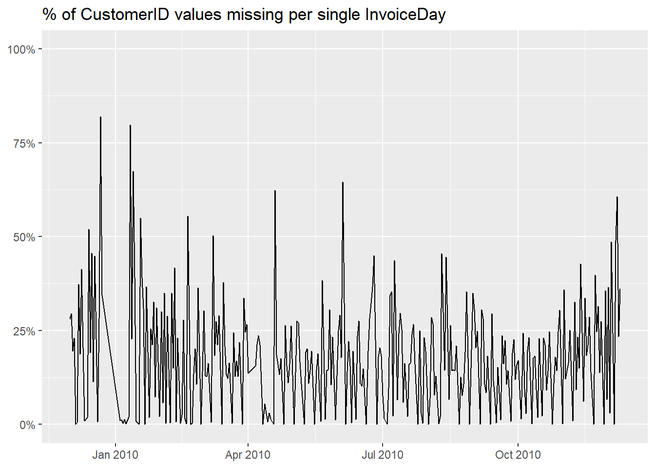
The graph shows us that the lack of CustomerID is very
distributed along the temporal dimension of our data frame, with some
spikes on specific days. We have 20% of missing values so
we could expect it.
- Country
About the missing values in the Country column, much
less diffused as they amount to only 308 rows,
df_cleaned %>%
  filter(is.na(Country))
they are present for just 4 customers,
df_cleaned %>%
  filter(is.na(Country)) %>%
  count(CustomerID, name = "Number of Occurrences")
and 13 invoices, most of which confirmed.
df_cleaned %>%
  filter(is.na(Country)) %>%
  count(Invoice, sort = TRUE, name = "Number of Purchases")
These customers never had a Country value in this data
frame, so we can’t impute them.
df_cleaned %>%
  filter(is.na(Country) &
           !is.na(CustomerID)) %>%
  count(CustomerID, Country, name = "Number of Occurrences")
There doesn’t seem to be a particular item
df_cleaned %>%
  group_by(StockCode, Description) %>%
  summarize("Percentage of NAs" = formattable::percent(mean(is.na(Country))),
            "Number of Occurrences" = n(), .groups = "drop") %>%
  arrange(desc(`Percentage of NAs`))
or a Quantity
df_cleaned %>%
  group_by(Quantity) %>%
  summarize("Percentage of NAs" = formattable::percent(mean(is.na(Country))),
            "Number of Occurrences" = n(), .groups = "drop") %>%
  arrange(desc(`Percentage of NAs`))
or Price
df_cleaned %>%
  group_by(Price) %>%
  summarize("Percentage of NAs" = formattable::percent(mean(is.na(Country))),
            "Number of Occurrences" = n(), .groups = "drop") %>%
  arrange(desc(`Percentage of NAs`))
value for which the NAs in the Country
column are evidently more frequent.
On the time scale, this is where NAs are located.
df_cleaned %>%
  filter(is.na(Country)) %>%
  group_by(Invoice, "Invoice Day" = as.Date(InvoiceDate)) %>%
  summarise("Number of Purchases" = n(), .groups = "drop") %>%
  arrange(`Invoice Day`)
df_cleaned %>%
  group_by(InvoiceDay = as.Date(InvoiceDate)) %>%
  summarize(N = sum(is.na(Country))) %>%
  ggplot(aes(InvoiceDay, N)) +
  geom_line() +
  labs(x = NULL,
       y = NULL,
       title = "Number of Country values missing per single InvoiceDay")
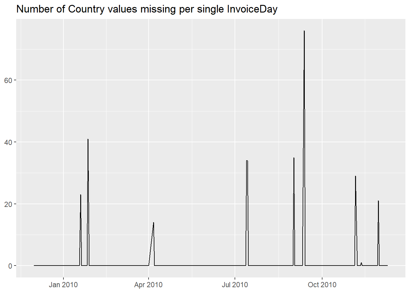
Final observation, there are 30 rows where we have
NAs in both the CustomerID and
Country columns.
df_cleaned %>%
  filter(is.na(CustomerID) &
           is.na(Country))
- duplicated rows
Sometimes we might have rows that are duplicated; as an example we
show the repetitions for the stock codes 21491 and
21912, occurring in invoice 489517.
df_cleaned %>%
  filter(Invoice == "489517" &
           StockCode %in% c("21491", "21912"))
We can easily remove the duplicated rows after the first,
df_cleaned %>%
  filter(Invoice == "489517" &
           StockCode %in% c("21491", "21912")) %>%
  distinct()
and doing that on all the data frame we notice that we lose
6853 rows, roughly the 1%.
tibble("with Duplicated Rows" = nrow(df_cleaned),
       "w/o Duplicated Rows" = df_cleaned %>%
         distinct() %>%
         nrow(),
       "Difference" = `with Duplicated Rows` - `w/o Duplicated Rows`,
       "Percentage" = formattable::percent(Difference / `with Duplicated Rows`))
We can inspect the removed rows,
df_cleaned %>%
  count(across(everything()), name = "Number of Occurrences") %>%
  filter(`Number of Occurrences` > 1) %>%
  arrange(InvoiceDate)
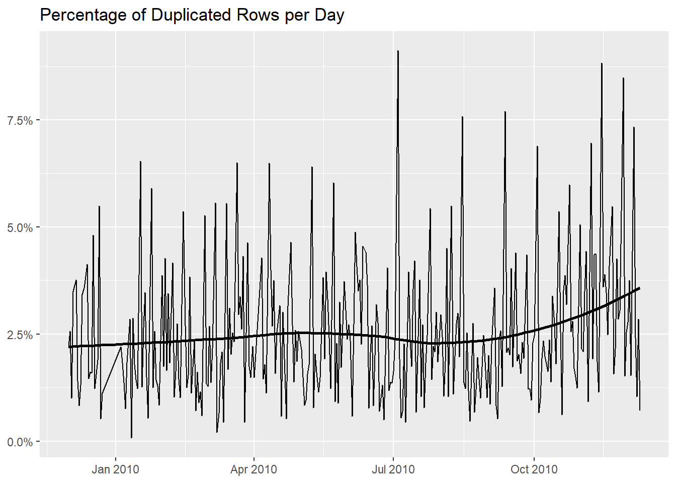
to see if they are present during certain condition, usually at a
specific time stamp, and we see that at the end of 2010
they are slightly more frequent, as shown by the horizontal line that
represents the trend (do recall though that we have a significant upward
one of invoices per day).
library(ggplot2)
df_cleaned %>%
  count(across(everything()), name = "Number of Occurrences") %>%
  mutate(Status = if_else(`Number of Occurrences` > 1, "Repetition", "Not A Repetition"),
         InvoiceDay = as.Date(InvoiceDate)) %>%
  group_by(InvoiceDay, Status) %>%
  summarise(n = sum(`Number of Occurrences`), .groups = "drop_last") %>%
  mutate(Percentage = n / sum(n)) %>%
  ungroup() %>%
  filter(Status == "Repetition") %>%
  ggplot(aes(InvoiceDay, Percentage)) +
  geom_line() +
  geom_smooth(formula = y ~ x, method = "loess", color = "black", se = FALSE) +
  scale_y_continuous(labels = scales::label_percent()) +
  labs(x = NULL,
       y = NULL,
       title = "Percentage of Duplicated Rows per Day")
To advance an hypothesis, we recall invoice 489517, an
invoice with 38 rows, 8 of which are
duplicated one or several times.
df_cleaned %>%
  filter(Invoice == "489517") %>%
  group_by(across(everything())) %>%
  mutate("Number of Occurrences" = n()) %>%
  ungroup() %>%
  arrange(StockCode)
We suggest that it could also be possible that, given the nature of
this data frame, those are not duplicated rows but just purchases that
has been imputed several times without aggregating them. Here for
example stock code 21491 might have had just one row with
2 for Quantity.
df_cleaned %>%
  filter(Invoice == "489517" &
           StockCode == "21491")
In the same way as stock code 21790 has one row with
4 and another with 1.
df_cleaned %>%
  filter(Invoice == "489517" &
           StockCode == "21790")
So erasing them might not be a good option as we would lose
information about Quantity.
If we were to remove also the rows like the one for stock code
21790, where we only have a difference in the
Quantity column, we would lose 5985 additional
rows.
tibble("w/o Duplicated Rows" = df_cleaned %>%
         distinct() %>%
         nrow(),
       "w/o Different Quantity Rows" = df_cleaned %>%
         group_by(pick(!Quantity)) %>%
         slice(1) %>%
         ungroup() %>%
         nrow(),
       "Difference" = `w/o Duplicated Rows` - `w/o Different Quantity Rows`)
We could therefore merge these lines in case we are considering that
are not duplicated.
df_cleaned %>%
  group_by(across(c(-Quantity))) %>%
  summarise(Quantity = sum(Quantity), .groups = "drop") %>%
  filter(Invoice == "489517") %>%
  relocate(Quantity, .after = Description)
The data frame presents various cases like these, where we have the
same stock code with a different quantity in the same invoice,
df %>%
  count(Invoice, StockCode, wt = n_distinct(Quantity), name = "Number of Occurrences") %>%
  filter(`Number of Occurrences` > 1)
but also stock codes with different prices in the same invoice, like
here
df %>%
  filter(Invoice == "489560" &
           StockCode == "35955")
albeit this phenomenon is less frequent,
df %>%
  count(Invoice, StockCode, wt = n_distinct(Price), name = "Number of Occurrences") %>%
  filter(`Number of Occurrences` > 1)
and can be more easily explained by different unit prices for
different volumes of purchases, although it happening in the same
invoice is rather odd.