In this document we will present the data frame used throughout this
site, with the mean to have a first understanding of its structure and
characteristics.
- source and structure
The data frame was first retrieved, on the 1st of September 2022,
from https://archive.ics.uci.edu/ml/datasets/Online+Retail+II
and its description states that
“This Online Retail II data set contains all the transactions
occurring for a UK-based and registered, non-store online retail between
01/12/2009 and 09/12/2011.The company mainly sells unique all-occasion
gift-ware. Many customers of the company are wholesalers.”
The data frame consists of 525461 rows and of these
8 columns, whose class is correct,
library(dplyr)
df %>%
  summarise(across(everything(), ~ class(.x)[1]))
except for Customer ID, that we will transform into
character, removing the empty space from the name as well.
df <- df %>%
  mutate(CustomerID = as.character(`Customer ID`), .keep = "unused", .after = Price)
The data frame looks like this:
Where we can see that each row contains information about the
purchase of an item.
The rows are ordered by InvoiceDate, so all the
purchases pertaining to a single Invoice are adjacent.
- checking for tidiness
We see how the data frame respects the three rules of tidy data
(every column is a variable, every row is an observation, every cell is
a single value). This avoids the need to manipulate the rows and columns
before proceeding into successive steps.
- respect of the definitions
In this section we will examine whether or not the data frame
respects the definitions stated in the web page it was retrieved
from.
- Invoice
Invoice is defined as
“Invoice number. Nominal. A 6-digit integral number uniquely assigned
to each transaction. If this code starts with the letter ‘c’, it
indicates a cancellation.”
There are 28816 distinct invoices.
library(knitr)
kable(df %>%
        distinct(Invoice) %>%
        tally(name = "Number of Distinct Invoices"), align = "l")
4592 of which have been cancelled, the
15.94%.
library(stringr)
df %>%
  mutate(Status = if_else(str_starts(Invoice, "C"), "Cancelled", "Confirmed")) %>%
  group_by(Status) %>%
  summarize("Number of Distinct Invoices" = n_distinct(Invoice)) %>%
  mutate(Percentage = formattable::percent(`Number of Distinct Invoices` / sum(`Number of Distinct Invoices`))) %>%
  arrange(desc(`Number of Distinct Invoices`))
We confirm that every Invoice is related to just one customer.
kable(df %>%
        count(Invoice, wt = n_distinct(CustomerID), name = "Number of Customers") %>%
        filter(`Number of Customers` > 1) %>%
        tally(`Number of Customers`, name = "Number of Invoices with more than one Customer"), align = "l")
There are some invoices that don’t start with C
though.
df %>%
  filter(str_length(Invoice) != 6 &
           !str_starts(Invoice, "C"))
- StockCode
StockCode is defined as
“Product (item) code. Nominal. A 5-digit integral number uniquely
assigned to each distinct product.”
In the time frame of the data, 4631 different items
have been invoiced.
kable(df %>%
        distinct(StockCode) %>%
        tally(name = "Number of Distinct Stock Codes"), align = "l")
Not all the stock codes are numbers of length 5
though.
df %>%
  filter(str_length(StockCode) != 5)
Nor they seem perfectly uniquely assigned.
df %>%
  count(StockCode, Description, name = "Number of Occurrences") %>%
  group_by(StockCode) %>%
  filter(n() > 1) %>%
  ungroup()
- Description
Description is defined as
“Product (item) name. Nominal.”
and there are 4644 distinct ones, a number
different from the distinct stock codes (when instead they should be
equal), owing to multiple descriptions for some of them, as we’ve seen a
little above.
kable(df %>%
        distinct(Description) %>%
        tally(name = "Number of Distinct Descriptions"), align = "l")
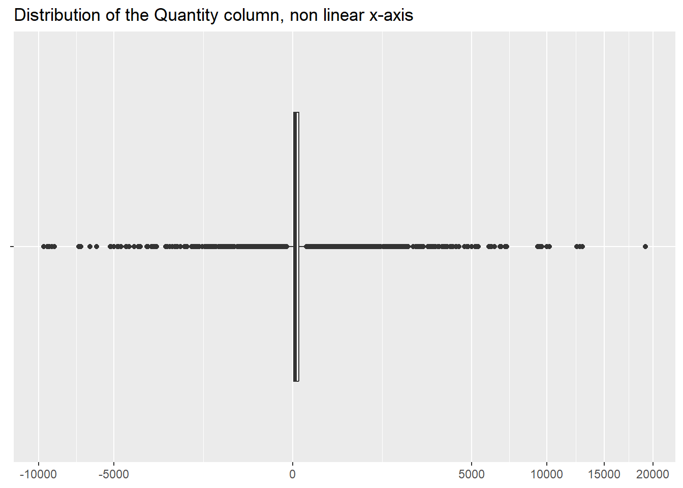
- Quantity
Quantity is defined as
“The quantities of each product (item) per transaction. Numeric.”
Looking at its distribution, we can see that most items are sold
in small quantities, but there are larger values as well, both negative
and positive.
df %>%
  reframe(Value = summary(Quantity))  %>%
  mutate(Statistic = c("Min.", "1st Qu.", "Median", "Mean", "3rd Qu.", "Max"), .before = Value)
library(ggplot2)
ggplot(df, aes(Quantity, "")) +
  geom_boxplot() +
  scale_x_continuous(trans = scales::modulus_trans(0.5), breaks = scales::breaks_extended(n = 9)) +
  labs(x = NULL,
       y = NULL,
       title ="Distribution of the Quantity column, non linear x-axis")
- InvoiceDate
InvoiceDate is defined as
“Invoice date and time. Numeric. The day and time when a transaction
was generated.”
Here we can take a look at how wide our time frame is and at how
many invoices per day there are.
df %>%
  group_by("Invoice Day" = as.Date(InvoiceDate)) %>%
  mutate("Number of Invoices" = n_distinct(Invoice)) %>%
  ungroup() %>%
  ggplot(aes(`Invoice Day`, `Number of Invoices`)) +
  geom_line() +
  labs(x = "",
       y = "",
       title = "Number of Invoices per Day")
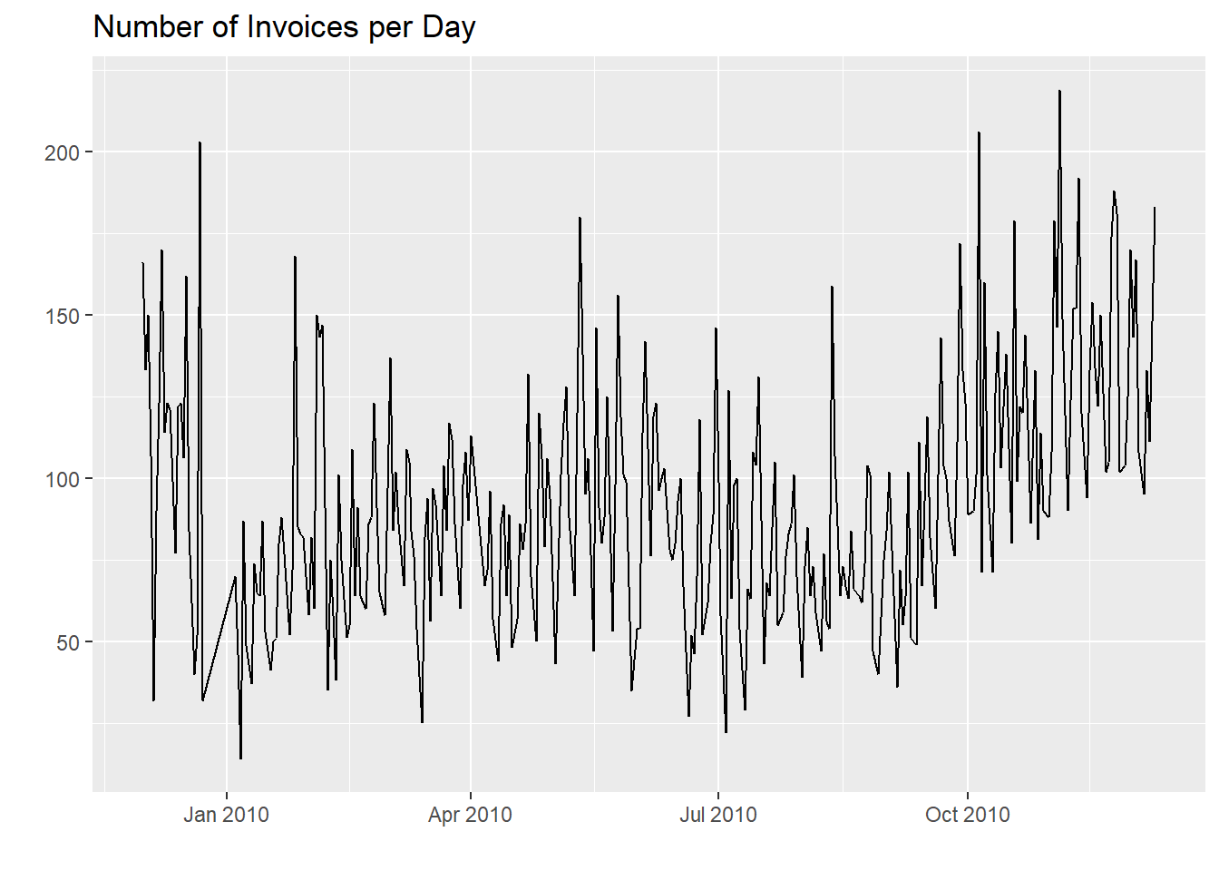
We notice that the last day is not 09/12/2011 as stated
in the data frame definition but one year prior
(09/12/2010),
kable(tibble("Last Day Present in the Data Frame" = max(as.Date(df$InvoiceDate))), align = "l")
for a total of 373 days.
kable(tibble("Time Span" = max(as.Date(df$InvoiceDate)) - min(as.Date(df$InvoiceDate))), align = "l")
- Price
Price is defined as
“Unit price. Numeric. Product price per unit in sterling (£).”
As per Quantity, we will take a look at its
distribution.
df %>%
  reframe(Value = summary(Price))  %>%
  mutate(Statistic = c("Min.", "1st Qu.", "Median", "Mean", "3rd Qu.", "Max"), .before = Value)
ggplot(df, aes(Price, "")) +
  geom_boxplot() +
  scale_x_continuous(trans = scales::modulus_trans(0.25)) +
  labs(x = NULL,
       y = NULL,
       title ="Distribution of the Price column, non linear x-axis")
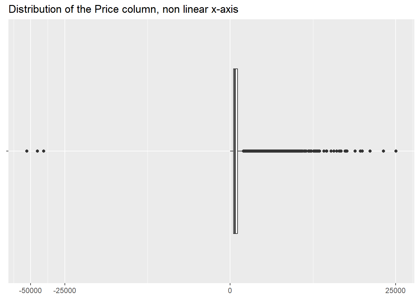
Here we gather that the items we sell are largely cheap with some
outliers, both positive and negative.
- Customer ID
Customer ID (previously changed to
CustomerID) is defined as
“Customer number. Nominal. A 5-digit integral number uniquely
assigned to each customer.”
There are 4384 different customers in our data
frame.
kable(df %>%
        distinct(CustomerID) %>%
        tally(name = "Number of Distinct Customers"), align = "l")
- Country
Country is defined as
“Country name. Nominal. The name of the country where a customer
resides.”
The customers are from 40 different countries,
mostly European ones.
We notice as well an Unspecified value, occurring for
6 customers.
df %>%
  count(Country, wt = n_distinct(CustomerID), sort = TRUE, name = "Number of Customers")
- main takeaways
Besides gaining a general knowledge about the data frame, that we can
sum up in the following table,
df %>%
  summarise(across(where(is.character), n_distinct),
            across(where(is.numeric), median))
where we showed the number of distinct values for the characters
columns and the median value for the numeric ones, we have assembled
some points of interest we will investigate, among other things, during
the Data Wrangling sections.
Those are:
- the
Invoice column contains values that don’t start
with C
- the
Stockcode column’s values don’t respect the
definition
- the non univocal relation between
StockCode and
Description
- the time frame is one year shorter than stated
Unspecified values in the Country
column