Data wrangling is a set of procedures aimed at “cleaning” a data
frame, removing inconsistencies, typos and mistakes, to prepare a solid
ground for future analysis.
The mindset that will guide us here will be to remove rows that don’t
pertain to real transactions between the retailer and the customers.
Building up from our previous document, we will start by checking,
for every column, if the definitions stated in the source are
respected.
- Invoice
The first definition determines that, if an invoice starts with
C, like C489449, it means that it has been
cancelled.
But we can also find values that start with a letter different that
C.
library(stringr)
df %>%
  filter(str_length(Invoice) != 6 &
           !str_starts(Invoice, "C"))
Invoices that don’t seem to be actual transactions with a customer,
so we will remove them.
- StockCode
About the stock codes, not all of them are “5-digit integral
number”.
df %>%
  filter(str_length(StockCode) != 5)
Among those, values like 79323P and 79323W
are actual transactions and must be kept.
From the remaining 77 values,
df %>%
  filter(str_length(StockCode) != 5 &
           !str_detect(StockCode, "^\\d{5}[a-zA-Z]{1,2}$")) %>%
  count(StockCode, Description, sort = TRUE, name = "Number of Occurrences")
we will keep PADS and the values starting with
DCGS, SP or gift, leaving us with
2900 rows to remove from the data frame.
df %>%
  filter(str_length(StockCode) != 5 &
           !str_detect(StockCode, "^\\d{5}[a-zA-Z]{1,2}$") &
           !str_detect(StockCode, "PADS|DCGS|SP|gift"))
- D for Discount
About D, that stands for Discount, we
follow the common understanding that, under certain conditions, a
discount is applied to an invoice to lower its total amount, and already
we notice that none of the Discount stock codes have a
negative value, as one should expect, in the Price
column.
library(knitr)
kable(df %>%
        filter(StockCode == "D" &
                 Price < 0) %>%
        tally(name = "Number of `Discount` Stock Codes with a Negative Price"), align = "l")
It could be the case though that the discount is applied through the
negative value in the Quantity column (multiplying
Quantity per Price), but there are as well
5 purchases with a positive value in it.
df %>%
  filter(StockCode == "D") %>%
  count("Negative Quantity" = if_else(Quantity < 0, "Yes", "No"))
The negative values pertain to cancelled invoices while the positive
ones to confirmed ones.
df %>%
  filter(StockCode == "D") %>%
  count("Negative Quantity" = if_else(Quantity < 0, "Yes", "No"),
        Status = if_else(str_starts(Invoice, "C"), "Cancelled", "Confirmed")
        , name = "Number of Invoices")
Overall there are 90 invoices, 85 cancelled
and 5 confirmed, with at least one row with
StockCode equal to D,
df %>%
  group_by(Invoice) %>%
  filter(any(StockCode == "D")) %>%
  summarise(n = n()) %>%
  count(Status = if_else(str_starts(Invoice, "C"), "Cancelled", "Confirmed"), name = "Number of Invoices")
for a total of 131 rows.
df %>%
  group_by(Invoice) %>%
  filter(any(StockCode == "D")) %>%
  ungroup()
81 of those are single line invoices, so we don’t
understand what they should have discounted.
df %>%
  group_by(Invoice) %>%
  filter(any(StockCode == "D")) %>%
  summarise("Number of Items" = n()) %>%
  count(`Number of Items`, sort = TRUE, name = "Number of Occurrences")
Maybe it’s a discount on a previous invoice, but we wouldn’t know how
to connect them together, plus 76 out of those
81 single line invoices have been cancelled as well.
df %>%
  group_by(Invoice) %>%
  filter(any(StockCode == "D") &
           n() == 1) %>%
  ungroup() %>%
  count("Status of Single Line Invoices" = if_else(str_starts(Invoice, "C"), "Cancelled", "Confirmed"), name = "Number of Invoices")
The 5 that have not been cancelled have, like all the
others, a positive value in the Price column and that,
putting aside a mistake that can be easily fixed, begs the question on
whether D (Discount) is an article that can be
bought and then redeemed later, like a voucher, but, as we can see in a
previous table, we already have the gift_xxxx_xx stock code
for that (unless that is specific to Dotcomgiftshop).
df %>%
  group_by(Invoice) %>%
  filter(any(StockCode == "D") &
           !str_starts(Invoice, "C")) %>%
  ungroup()
About the 9 invoices with more than one line,
df %>%
  group_by(Invoice) %>%
  filter(any(StockCode == "D") &
           n() > 1) %>%
  ungroup()
for 3 of them it is always D the stock
code.
df %>%
  group_by(Invoice) %>%
  filter(all(StockCode == "D") &
           n() > 1) %>%
  ungroup()
The 6 remaining can be investigated further, at a first
glance we can see that they all have been cancelled.
df %>%
  group_by(Invoice) %>%
  filter(any(StockCode == "D") &
           n() > 1) %>%
  ungroup() %>%
  anti_join(df %>%
              group_by(Invoice) %>%
              filter(all(StockCode == "D") &
                       n() > 1) %>%
              ungroup(), by = "Invoice")
Incidentally the value of discounts in percentage is very high for
some of them, it seems more like a refund plus eventual fines.
df %>%
  group_by(Invoice) %>%
  filter(any(StockCode == "D") &
           n() > 1) %>%
  ungroup() %>%
  anti_join(df %>%
              group_by(Invoice) %>%
              filter(all(StockCode == "D") &
                       n() > 1) %>%
              ungroup(), by = "Invoice") %>%
  mutate(Status = if_else(str_detect(StockCode, "D"), "Discount", "Purchases")) %>%
  group_by(Invoice, Status) %>%
  summarise("Value in £" = sum(abs(Quantity * Price)), .groups = "drop_last") %>%
  mutate("Discount Percentage" = formattable::percent(if_else(Status == "Discount",
                                                              `Value in £`[Status == "Discount"] / `Value in £`[Status == "Purchases"],
                                                              NA))) %>%
  arrange(desc(Status), .by_group = TRUE) %>%
  ungroup()
Considering everything, how few valuable information we could extract
from the rows that with D as a stock code and that there
are only 131 of them (out of 525461), we
decide to remove them.
- Description
Another discrepancy is in the different number of distinct stock
codes and descriptions, that should be the same.
df %>%
  summarise("Number of Distinct Stock Codes" = n_distinct(StockCode),
            "Number of Distinct Descriptions" = n_distinct(Description))
That is because some stock codes (2003 out of
4631) have several descriptions,
kable(df %>%
        count(StockCode, Description, name = "Number of Occurrences") %>%
        group_by(StockCode) %>%
        filter(n() > 1) %>%
        group_keys() %>%
        tally(name = "Number of Stockcodes with several Descriptions"), align = "l")
of various nature.
df %>%
  count(StockCode, Description, name = "Number of Occurrences") %>%
  group_by(StockCode) %>%
  filter(n() > 1) %>%
  ungroup()
For 1564 out of those 2003 an additional
description is a missing value (NA).
kable(df %>%
        count(StockCode, Description, name = "Number of Occurrences") %>%
        group_by(StockCode) %>%
        filter(n() > 1) %>%
        semi_join(df %>%
                    count(StockCode, Description) %>%
                    group_by(StockCode) %>%
                    filter(any(is.na(Description))) %>%
                    ungroup(), by = "StockCode") %>%
        group_keys() %>%
        tally(name = "Number of Stockcodes with NA as Description"), align = "l")
df %>%
  count(StockCode, Description, name = "Number of Occurrences") %>%
  group_by(StockCode) %>%
  filter(n() > 1) %>%
  ungroup() %>%
  semi_join(df %>%
              count(StockCode, Description) %>%
              group_by(StockCode) %>%
              filter(any(is.na(Description))) %>%
              ungroup(), by = "StockCode")
While the others 439 present typos, updated descriptions
or notes.
kable(df %>%
        count(StockCode, Description, name = "Number of Occurrences") %>%
        group_by(StockCode) %>%
        filter(n() > 1) %>%
        anti_join(df %>%
                    count(StockCode, Description) %>%
                    group_by(StockCode) %>%
                    filter(any(is.na(Description))) %>%
                    ungroup(), by = "StockCode") %>%
        group_keys() %>%
        tally(name = "Stockcodes with diverse Descriptions"), align = "l")
df %>%
  count(StockCode, Description, name = "Number of Occurrences") %>%
  group_by(StockCode) %>%
  filter(n() > 1) %>%
  ungroup() %>%
  anti_join(df %>%
              count(StockCode, Description) %>%
              group_by(StockCode) %>%
              filter(any(is.na(Description))) %>%
              ungroup(), by = "StockCode")
The notes are usually written in lower case.
df %>%
  count(StockCode, Description, name = "Number of Occurrences") %>%
  group_by(StockCode) %>%
  filter(n() > 1) %>%
  ungroup() %>%
  anti_join(df %>%
              count(StockCode, Description) %>%
              group_by(StockCode) %>%
              filter(any(is.na(Description))) %>%
              ungroup(), by = "StockCode") %>%
  filter(str_detect(Description, "[:lower:]"))
Furthermore, also amongst the stock code with only one description we
experience some issues, like NAs values and notes.
df %>%
  count(StockCode, Description, name = "Number of Occurrences") %>%
  group_by(StockCode) %>%
  filter(n() == 1 &
           (is.na(Description) |
              str_detect(Description, "[:lower:]")))
We can also encounter the same description pertaining to different
stock codes; some they just differ in style
df %>%
  count(Description, StockCode, name = "Number of Occurrences") %>%
  group_by(Description) %>%
  filter(n() > 1 &
           str_length(StockCode) != 5 &
           !str_detect(Description, "[:lower:]")) %>%
  ungroup()
while others are two different ones.
df %>%
  count(Description, StockCode, name = "Number of Occurrences") %>%
  filter(Description != "?") %>%
  group_by(Description) %>%
  filter(n() > 1 &
           str_length(StockCode) == 5 &
           !str_detect(Description, "[:lower:]")) %>%
  ungroup()
So we might say that Description is not a column we can
rely on too much.
- Quantity
Moving on to Quantity, let’s investigate the purchases
with a negative value of it,
df %>%
  filter(Quantity < 0)
that amount to 12326 of them,
kable(df %>%
        filter(Quantity < 0) %>%
        tally(name = "Purchases with a negative Quantity"), align = "l")
belonging to 6712 invoices, out of which
4591 are cancelled, and for them it makes sense that the
quantity is negative, as a way to readjust the inventory levels of the
stock code.
df %>%
  group_by(Invoice) %>%
  filter(any(Quantity < 0)) %>%
  ungroup() %>%
  distinct(Invoice) %>%
  count(Status = if_else(str_starts(Invoice, "C"), "Cancelled", "Confirmed"), name = "Number of Invoices")
But the rest are not cancelled and they seem to have some common
concurrences,
df %>%
  filter(Quantity < 0 &
           !str_detect(Invoice, "C"))
besides being all single line invoices,
kable(df %>%
        filter(Quantity < 0 &
                 !str_detect(Invoice, "C")) %>%
        group_by(Invoice) %>%
        filter(n() > 1) %>%
        ungroup() %>%
        tally(name = "Number of Confirmed Negative Quantity Invoices with more than One Line"), align = "l")
like NAs or notes in the Description
column,
df %>%
  filter(Quantity < 0 &
           !str_detect(Invoice, "C")) %>%
  count(Description, sort = TRUE, name = "Number of Occurrences")
and with all the same value in the Price,
CustomerID and Country columns.
df %>%
  filter(Quantity < 0 &
           !str_detect(Invoice, "C")) %>%
  distinct(Price, CustomerID, Country)
These invoices run through all the data frame so the issue is not
time specific.
library(ggplot2)
df %>%
  filter(Quantity < 0 &
           !str_detect(Invoice, "C")) %>%
  ggplot(aes(InvoiceDate, 5)) +
  geom_point() +
  labs(x = NULL,
       y = NULL,
       title = "Time Placement of Confirmed Invoices with a Negative Quantity") +
  theme(axis.text.y = element_blank(),
        axis.ticks.y = element_blank())
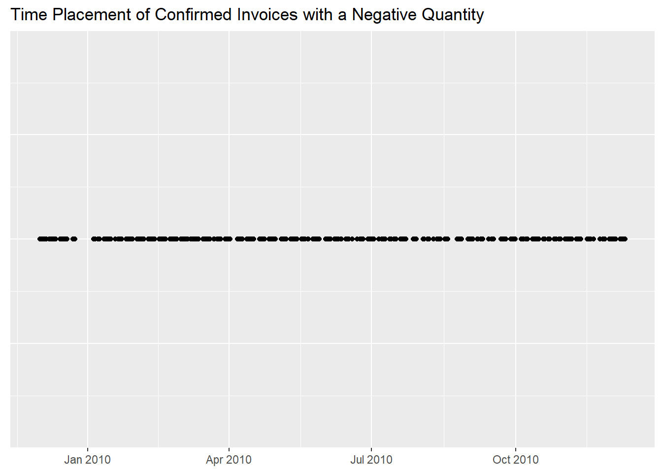
We can assume that these are not actual transactions but inventory
adjustments, so we will remove them.
We’ve seen that, when an invoice has a C, its quantity
is negative but there is one case where that is not true.
df %>%
  filter(str_detect(Invoice, "C") &
           Quantity >= 0)
There are no values equal to 0,
kable(df %>%
        filter(Quantity == 0) %>%
        tally(name = "Number of Rows with 0 Quantity"), align = "l")
and no invoices with both positive and negative ones.
kable(df %>%
        mutate(class = if_else(Quantity > 0, "Positive Quantity", "Negative Quantity")) %>%
        count(Invoice, class) %>%
        group_by(Invoice) %>%
        filter(n() > 1) %>%
        ungroup() %>%
        tally(name = "Number of Invoices with Both Positive and Negative Quantity Values"), align = "l")
- InvoiceDate
About InvoiceDate, let’s look for gaps.
date_range <- seq(min(as.Date(df$InvoiceDate)), max(as.Date(df$InvoiceDate)), by = 1)
gaps <- tibble("Missing Days" = date_range[!date_range %in% as.Date(df$InvoiceDate)])
ggplot(gaps, aes(`Missing Days`, 5)) +
  geom_point() +
  labs(x = NULL,
       y = NULL,
       title = "Missing days during our time span") +
  theme(axis.text.y = element_blank(),
        axis.ticks.y = element_blank())
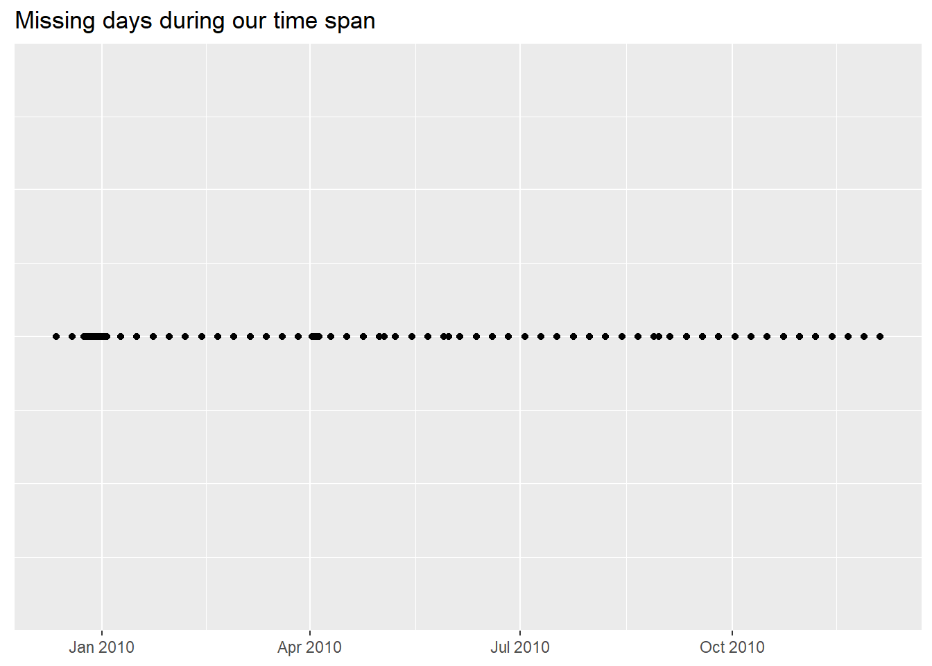
There is a large sequence of missing days around
Christmas 2009 and a smaller one at the beginning of
April 2010 (Easter fell on the 4th of April
that year) but those are not the only ones missing.
tibble("Missing Day" = date_range[!date_range %in% as.Date(df$InvoiceDate)],
       "Day of the Week" = weekdays(date_range[!date_range %in% as.Date(df$InvoiceDate)]))
If we count them we see that Saturday is the most
frequently missed.
tibble("Missing Days" = date_range[!date_range %in% as.Date(df$InvoiceDate)],
       "Day of the Week" = weekdays(date_range[!date_range %in% as.Date(df$InvoiceDate)])) %>%
  count(`Day of the Week`, sort = TRUE, name = "Number of Occurrences")
I was expecting Sunday to be honest given that the
clientele is mostly UK based. There might be other factors
at play here given the nature of the business.
- Price
Let’s look for abnormal prices now and for the negative ones we see
that they pertain to the invoices with an A.
And for the rows with a price equal to 0
(3687 of them),
df %>%
  filter(Price == 0)
they seem to be a superset of the ones with a negative quantity and a
not cancelled invoice (2121 rows, already seen in the Quantity section), that all had the same values in
the Price (0), CustomerID
(NA) and Country (United Kingdom)
columns.
df %>%
  filter(Quantity < 0 &
           !str_detect(Invoice, "C"))
Within the 1566 remaining rows of this set, that have a
positive Quantity,
df %>%
  filter(Price == 0 &
           Quantity > 0)
we similarly have missing values (NAs) in most of the
Description
df %>%
  filter(Price == 0 &
           Quantity > 0) %>%
  count(Description, sort = TRUE, name = "Number of Occurrences")
and CustomerID columns.
df %>%
  filter(Price == 0 &
           Quantity > 0) %>%
  count(CustomerID, sort = TRUE, name = "Number of Occurrences")
These purchases are not concentrated in particular time periods,
df %>%
  filter(Price == 0 &
           Quantity > 0) %>%
  ggplot(aes(InvoiceDate, 5)) +
  geom_point() +
  labs(x = NULL,
       y = NULL,
       title = "Time Placement of Purchases with Price equal to 0 and a positive Quantity") +
  theme(axis.text.y = element_blank(),
        axis.ticks.y = element_blank())
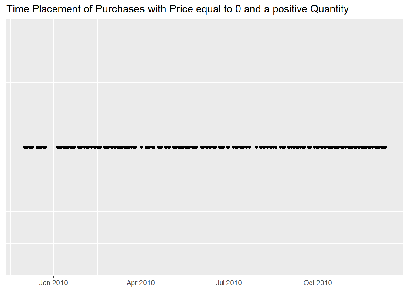
and they mostly pertain to United Kingdom.
df %>%
  filter(Price == 0 &
           Quantity > 0) %>%
  count(Country, sort = TRUE)
- CustomerID
About CustomerID, we have 5 customers, out
of 4384, that changed country but that is not a concern,
more something to keep in mind.
df %>%
  count(CustomerID, Country, name = "Number of Occurrences") %>%
  group_by(CustomerID) %>%
  filter(n() > 1 &
           !is.na(CustomerID)) %>%
  ungroup()
- Country
We noticed in the previous document the value
Unspecified for 15 invoices and 5
(plus NAs values) customers in the Country
column, that is better to change to NA.
df %>%
  filter(Country == "Unspecified") %>%
  distinct(Country, Invoice, CustomerID) %>%
  arrange(desc(CustomerID))
- main takeaways
Let’s recap our findings:
- Invoices starting with a letter different than
C
- Stock codes not pertaining to actual transactions
- A
D (Discount) stock code that doesn’t
provide valuable information
- A
Description column with several values
(NAs, typos, updated descriptions or notes) for the same
stock code, uninformative unique descriptions (NAs, notes)
for others, the same description assigned to different stock codes
2121 non cancelled invoices with a negative value in
the Quantity column, all with the same value in the
Price (0), CustomerID
(NA) and Country (United Kingdom)
columns, most likely inventory adjustments. 1 cancelled
invoice with a positive value in the Quantity column
- Unexpected gaps in the time frame
3 rows with a negative price (the same as the ones with
invoices starting with a letter different than C).
3687 rows with price equal to 0, a set
composed of rows with a negative (2121 rows) and with a
positive (1566) value in the Quantity
column5 customers that changed country
15 invoices and 5 customers with an
Unspecified value in the Country column
- resulting modifications
After these manipulations, the data frame has new
characteristics:
bind_rows("Cleaned Data Frame" = df_cleaned %>%
            summarise(across(where(is.character), n_distinct)),
          "Original Data Frame" = df %>%
            summarise(across(where(is.character), n_distinct)), .id = "")
- a different percentage of cancelled invoices, that increased to
16.64% from the previous 15.94%
bind_rows(df_cleaned %>%
            mutate(Status = if_else(str_starts(Invoice, "C"), "Cancelled", "Confirmed")) %>%
            group_by(Status) %>%
            summarize("Distinct Invoices" = n_distinct(Invoice)) %>%
            mutate("Percentage" = formattable::percent(`Distinct Invoices` / sum(`Distinct Invoices`))) %>%
            arrange(desc(`Distinct Invoices`)),
          df %>%
            mutate(Status = if_else(str_starts(Invoice, "C"), "Cancelled", "Confirmed")) %>%
            group_by(Status) %>%
            summarize("Distinct Invoices" = n_distinct(Invoice)) %>%
            mutate("Percentage" = formattable::percent(`Distinct Invoices` / sum(`Distinct Invoices`))) %>%
            arrange(desc(`Distinct Invoices`))) %>%
  mutate("Data Frame" = c("Cleaned", "", "Original", ""), .before = Status)
- and new distributions for the numeric columns, especially
Price.
bind_cols(df_cleaned %>%
            reframe(across(where(is.numeric), ~ summary(.x))) %>%
            rename("Cleaned Quantity" = Quantity, "Cleaned Price" = Price),
          df %>%
            reframe(across(where(is.numeric), ~ summary(.x))) %>%
            rename("Original Quantity" = Quantity, "Original Price" = Price)) %>%
  mutate("Statistic" = c("Min." , "1st Qu.", "Median", "Mean", "3rd Qu.", "Max.")) %>%
  relocate(Statistic, ends_with("y"), everything())
We notice that the gap between distinct stock codes and distinct
descriptions widened,
bind_rows("Cleaned Data Frame" = df_cleaned %>%
            summarise("Number of Distinct Stock Codes" = n_distinct(StockCode),
                      "Number of Distinct Descriptions" = n_distinct(Description)),
          "Original Data Frame" = df %>%
            summarise("Number of Distinct Stock Codes" = n_distinct(StockCode),
                      "Number of Distinct Descriptions" = n_distinct(Description)), .id = "")
despite we removed, from the Description column, all
missing values
kable(df_cleaned %>%
        filter(is.na(Description)) %>%
        tally(name = "Number of NAs in the Description Column"), align = "l")
and notes written in lower case.
df_cleaned %>%
  count(StockCode, Description, name = "Number of Occurrences") %>%
  filter(str_detect(Description, "[:lower:]"))
The number of invoices per day changed as well,
df_cleaned %>%
  group_by("Invoice Day" = as.Date(InvoiceDate)) %>%
  summarise("Cleaned Number of Invoices" = n_distinct(Invoice)) %>%
  left_join(df %>%
              group_by("Invoice Day" = as.Date(InvoiceDate)) %>%
              summarise("Original Number of Invoices" = n_distinct(Invoice)), by = "Invoice Day")
with a general decrease in number,
df_cleaned_plot <- df_cleaned %>%
  group_by("Invoice Day" = as.Date(InvoiceDate)) %>%
  mutate("Number of Invoices" = n_distinct(Invoice)) %>%
  ungroup()
colors <- c("Original" = "darkgrey",
            "Cleaned" = "black")
df %>%
  group_by("Invoice Day" = as.Date(InvoiceDate)) %>%
  mutate("Number of Invoices" = n_distinct(Invoice)) %>%
  ungroup() %>%
  ggplot(aes(`Invoice Day`, `Number of Invoices`)) +
  geom_line(aes(color = "Original")) +
  geom_line(data = df_cleaned_plot, aes(x = `Invoice Day`, y = `Number of Invoices`, color = "Cleaned")) +
  labs(x = "",
       y = "",
       title = "Number of Invoices per Day, differentiating by Data Frame",
       color = "Legend") +
  scale_color_manual(values = colors) +
  theme(legend.position = "bottom",
        legend.title = element_blank())
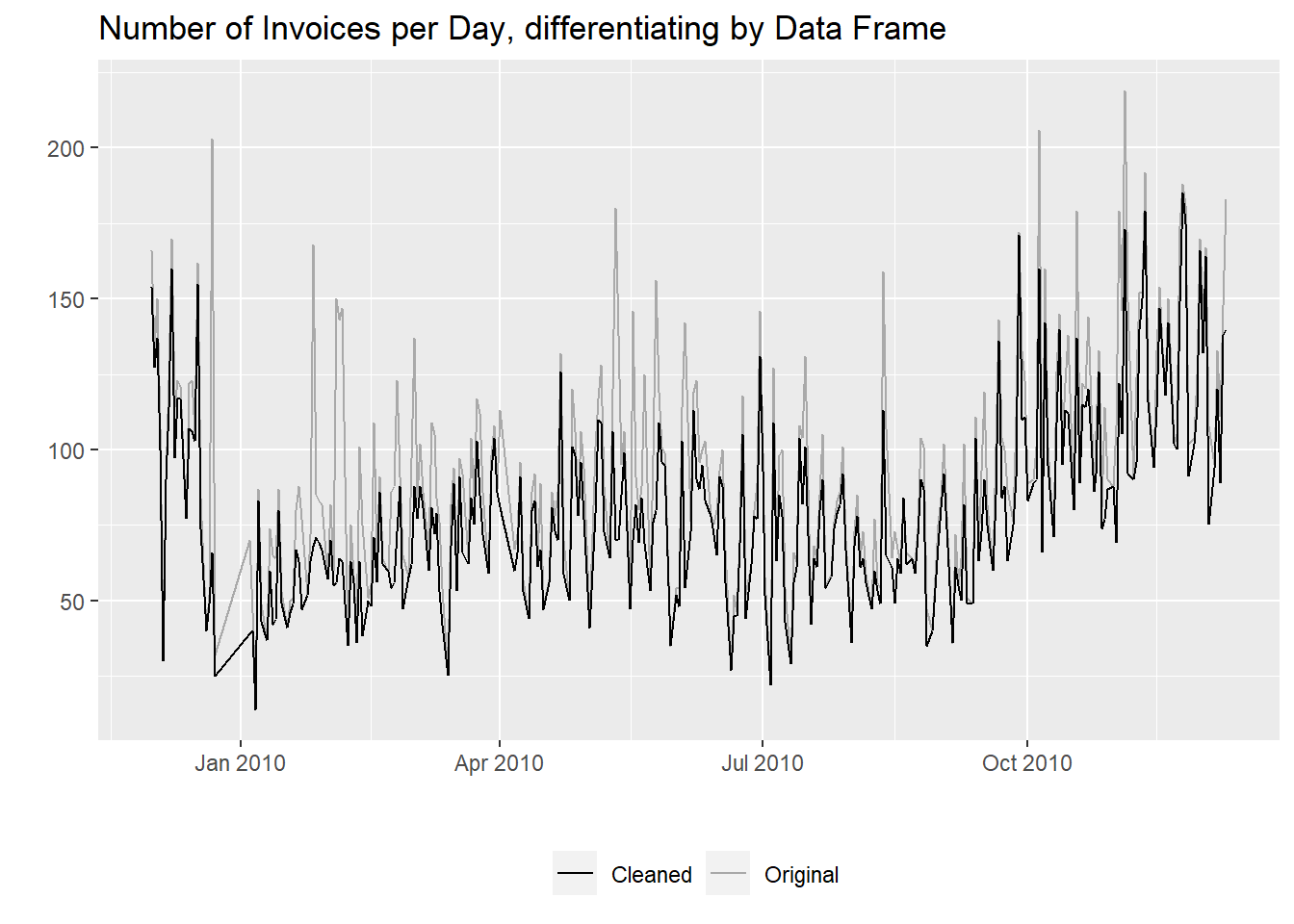
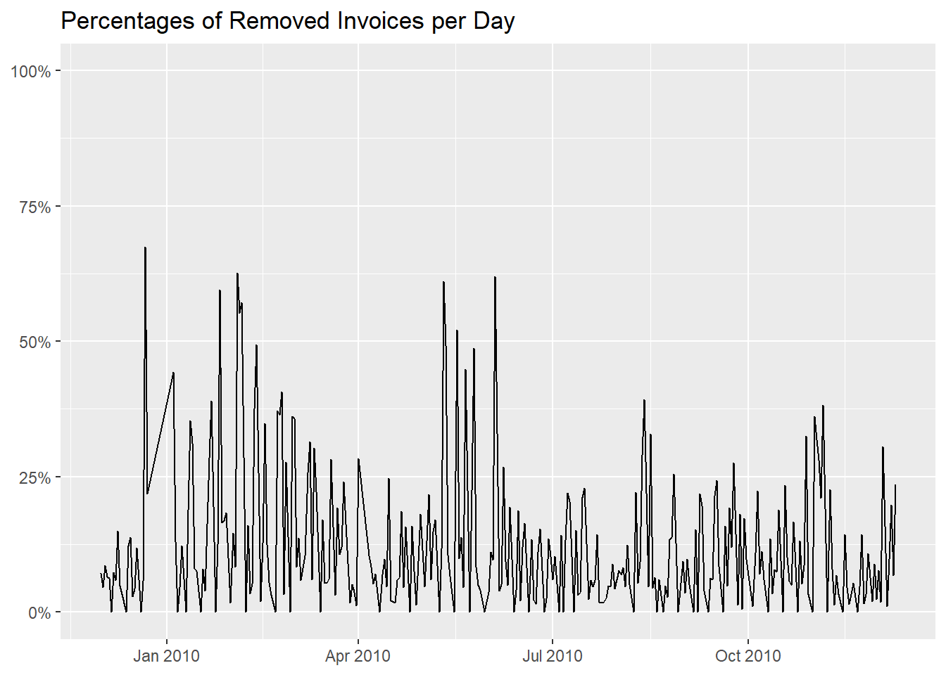
that is more relevant on certain days.
df_cleaned %>%
  group_by("Invoice Day" = as.Date(InvoiceDate)) %>%
  summarise("Cleaned Number of Invoices" = n_distinct(Invoice)) %>%
  left_join(df %>%
              group_by("Invoice Day" = as.Date(InvoiceDate)) %>%
              summarise("Original Number of Invoices" = n_distinct(Invoice)), by = "Invoice Day") %>%
  mutate(Percentage = abs((`Cleaned Number of Invoices` - `Original Number of Invoices`) / `Original Number of Invoices`)) %>%
  ggplot(aes(`Invoice Day`, Percentage)) +
  geom_line() +
  scale_y_continuous(labels = scales::label_percent(), limits = c(0, 1)) +
  labs(x = NULL,
       y = NULL,
       title = "Percentages of Removed Invoices per Day")
Furthermore, customer 12745 that was previously located
in two countries
df %>%
  count(CustomerID, Country, name = "Number of Occurrences") %>%
  group_by(CustomerID) %>%
  filter(n() > 1 &
           !is.na(CustomerID)) %>%
  ungroup()
is now exclusively in the United Kingdom.
df_cleaned %>%
  filter(CustomerID == "12745") %>%
  count(CustomerID, Country, name = "Number of Occurrences")
And of course the number of customers for each country changed.
df_cleaned %>%
  count(Country, wt = n_distinct(CustomerID), sort = TRUE, name = "Cleaned Data Frame") %>%
  full_join(df %>%
              count(Country, wt = n_distinct(CustomerID), name = "Original Data Frame"), by = "Country") %>%
  mutate(across(c(`Cleaned Data Frame`, `Original Data Frame`), ~ coalesce(as.character(.x), "not present")))