In this analysis we will divide our customers into different segments
based on their spending behaviors, not considering cancelled invoices
and removing as well the missing values in the CustomerID
column.
- preparations
We can, for example, model their spending behaviors with these
metrics.
(clustdf <- df %>%
   mutate(Expenses = Quantity * Price) %>%
   group_by(CustomerID) %>%
   summarise("Number of Invoices" = n_distinct(Invoice),
             "Number of Distinct Items Invoiced" = n_distinct(StockCode),
             "Total Quantity Purchased" = sum(Quantity),
             "Total of Expenses" = round(sum(Expenses), 2)) %>%
   left_join(df %>%
               mutate(Expenses = Quantity * Price) %>%
               group_by(CustomerID, Invoice) %>%
               summarise("Total Quantity per Invoice" = sum(Quantity),
                         "Total Expenses per Invoice" = sum(Expenses), .groups = "drop_last") %>%
               summarise("Rounded Median Quantity per Invoice" = round(median(`Total Quantity per Invoice`)),
                         "Rounded Median Revenues per Invoice" = round(median(`Total Expenses per Invoice`), 2)), by = "CustomerID"))
The algorithm we will use needs to know in advance how many segments
(clusters in its jargon) we want.
To determine their number, we can use graphical methods like the
following one,
set.seed(123)
#we set seeds as k-means may return different results for each run
clustdf_norm <- scale(clustdf[2:ncol(clustdf)])
#we z-score normalize the data to not have outliers influence the results
library(factoextra)
fviz_nbclust(clustdf_norm, kmeans, method = "wss", linecolor = "black") +
  labs(subtitle = "Elbow method")
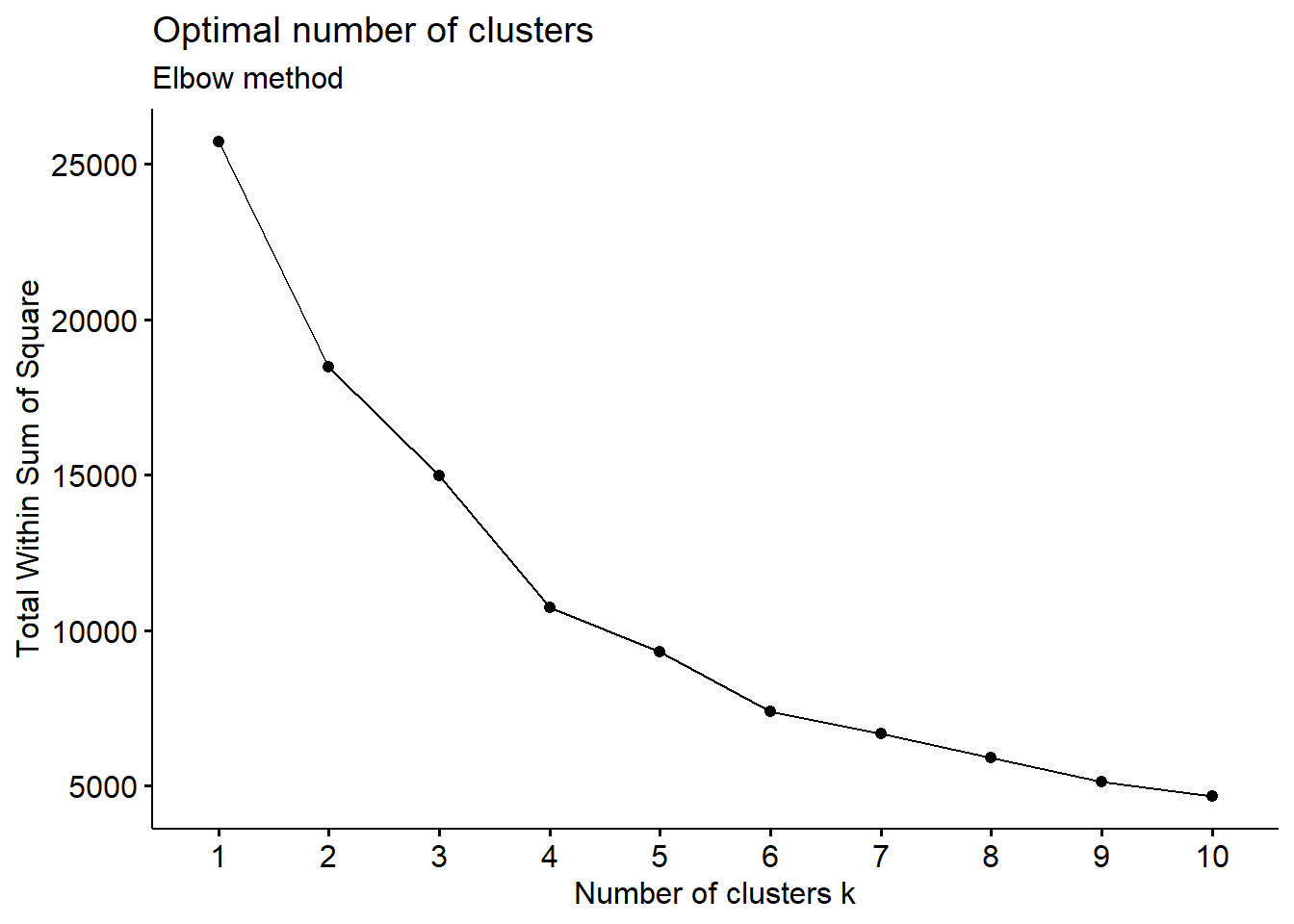
where we pick a value where the curve starts to get flat, meaning
that the decrements in value of the measure on the y axis are not
anymore significant as we increase the number of clusters.
We want that measure as small as possible, as it quantifies their
“compactness” as the “distances” between its members, so with smaller
distances we will have clusters that are more “closely-knit”, more
homogeneous.
With these premises, we choose 6 and we run the
algorithm.
set.seed(123)
kmclusters <- kmeans(clustdf_norm, centers = 6)
- analysis of results
The clusters returned by the algorithm are very different in size,
with one (number 1) that dominates.
knitr::kable(table(kmclusters$cluster), col.names = c("Cluster", "Number of Customers"))
| 1 |
3502 |
| 2 |
32 |
| 3 |
2 |
| 4 |
5 |
| 5 |
701 |
| 6 |
43 |
We can continue by analyzing their differences according to the
metrics designed at the beginning:
clustdf$Cluster <- kmclusters$cluster
df %>%
  left_join(clustdf %>%
              select(CustomerID, Cluster), by = "CustomerID") %>%
  mutate(Expenses = Quantity * Price) %>%
  group_by(Cluster) %>%
  summarise("Number of Invoices" = n_distinct(Invoice),
            "Number of Distinct Items Invoiced" = n_distinct(StockCode),
            "Total Quantity Purchased" = sum(Quantity),
            "Total of Expenses" = round(sum(Expenses), 2)) %>%
  left_join(df %>%
              left_join(clustdf %>%
                          select(CustomerID, Cluster), by = "CustomerID") %>%
              mutate(Expenses = Quantity * Price) %>%
              group_by(Cluster, Invoice) %>%
              summarise("Total Quantity per Invoice" = sum(Quantity),
                        "Total Expenses per Invoice" = sum(Expenses), .groups = "drop_last") %>%
              summarise("Rounded Median Quantity per Invoice" = round(median(`Total Quantity per Invoice`)),
                        "Rounded Median Revenues per Invoice" = round(median(`Total Expenses per Invoice`), 2)), by = "Cluster")
Cluster number 3 is surely interesting: only
2 customers (13687 and 13902),
for just 6 invoices, that contain large quantities of stock
codes and that yield high revenues.
df %>%
  left_join(clustdf %>%
              select(CustomerID, Cluster), by = "CustomerID") %>%
  filter(Cluster == 3)
Another topic of investigation can be the geographic
heterogeneity,
df %>%
  left_join(clustdf %>%
              select(CustomerID, Cluster), by = "CustomerID") %>%
  count(Cluster, wt = n_distinct(Country), name = "Number of Distinct Countries")
and clusters 2 and 4 seem rather restricted
in that regard (besides number 3, already examined).
df %>%
  left_join(clustdf %>%
              select(CustomerID, Cluster), by = "CustomerID") %>%
  filter(Cluster %in% c(2, 4)) %>%
  distinct(Cluster, Country) %>%
  arrange(Cluster)
Let’s see now if there are some clusters with few customers from the
UK (the country where more than 90% of them
reside),
df %>%
  left_join(clustdf %>%
              select(CustomerID, Cluster), by = "CustomerID") %>%
  distinct(Cluster, CustomerID, Country) %>%
  mutate(UK = if_else(Country == "United Kingdom", TRUE, FALSE)) %>%
  group_by(Cluster) %>%
  summarise("Percentage of UK Customers" = formattable::percent(mean(UK, na.rm = TRUE)))
and number 4 seems to be the one (there are only
5 customers in it though).
df %>%
  left_join(clustdf %>%
              select(CustomerID, Cluster), by = "CustomerID") %>%
  filter(Cluster == 4) %>%
  distinct(CustomerID, Country) %>%
  arrange(CustomerID)
Likewise, let’s see if there are clusters with mostly extra European
countries,
EU <-  c("Austria", "Belgium", "Channel Islands", "Cyprus", "Denmark", "EIRE", "Finland", "France", "Germany", "Greece", "Iceland", "Italy", "Lithuania", "Malta", "Netherlands", "Norway", "Poland", "Portugal", "Spain", "Sweden", "Switzerland", "United Kingdom")
df %>%
  left_join(clustdf %>%
              select(CustomerID, Cluster), by = "CustomerID") %>%
  distinct(Cluster, CustomerID, Country) %>%
  mutate(is_EU = if_else(Country %in% EU, TRUE, FALSE)) %>%
  group_by(Cluster) %>%
  summarise("Percentage of EU Customers" = formattable::percent(mean(is_EU, na.rm = TRUE)))
but that is not the case.
- main takeaways and further developments
In this first iteration of the application of a clustering algorithm
we grouped our clients into 6 different ones according to
some metrics meant to resume their spending behaviors. Following a brief
analysis of the results, we discovered two clients (13902
and 13687) with very peculiar ones.
Many more things can be done hereafter; we can change the number of
clusters to have either smaller or bigger groups, we can add, remove or
modify the metrics we designed, we can change the clustering algorithm
using one with different characteristics.